Sorry for my poor English. Please feel free to point out my mistakes. Many thanks.

Codeword and distance

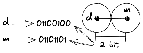
Before introducing the Hamming code, let’s take a brief look at the concept of codeword and distance. Consider the most classic ASCII encoding, where we represent a character with an 8-bit binary number, e.g. 01100100 for d, 01101101 for m, etc. Each group of 8 bits is called a codeword in this code space. At the same time, we can also define the distance between two codewords as the number of bits that differ between them. For example, the distance between 01100100 and 01101101 is 2. This distance is called Hamming distance or simply code distance.

Obviously, the distance between any two codewords of displayable characters is at least 1. If any one bit in the transmission is flipped, it will result in a different codeword, which places a demand on the reliability of the communication. One needs a way to add redundant information to the codeword so that the distance between the codewords is at least 2, to detect errors in the transmission. Apparently, this is not a textbook for coding, so I will not go into the details of various coding schemes, but only briefly introduce the Hamming code.

Hamming code

The Hamming code is a group error correction code proposed by Richard Wesley Hamming in 1950. The characteristic of the code is that any two codewords have a distance of at least 3. The idea is to add several redundant parity bits to the code to detect and correct 1-bit errors. The coding is as follows:

The Message row indicates each bit of the codeword. The Source row indicates whether the original value of the bit is data (Dx) or parity (Px). The Px row indicates which bits are parity-checked.

There is no restriction on the length of the original data in this encoding method, and the above table can be extended to meet the requirements of any length of data. However, the general encoding will discuss a specific length () for analytical convenience and simplicity. In the following, I will introduce two specific schemes, Hamming (7, 4) and Hamming (11, 7).

Hamming (7, 4)

The Hamming (7, 4) is a Hamming code with the encoded codeword length of 7 and the original data length of 4. It is encoded in the following way:

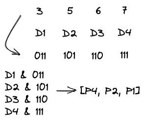
For each bit of the original data, the value of the parity bits is obtained by first performing a logical and operation with the binary representation of its position in the final message, and then performing a xor operation together.

Here is an example of data 1001 to demonstrate the encoding and error correction. According to the above process, we can write the parity bits [P4 P2 P1] = 011 ^ 111 = 100, and the final codeword is 0011001. Assuming an error in transmission, the received codeword is 0011101. We can calculate the parity bits in a similar way [P4 P2 P1] = 011 ^ 100 ^ 101 ^ 111 = 101, i.e. the 5th bit is flipped. We can correct the error by flipping the 5th bit back to 0 and getting the original data 1001.

We can also use matrixes to describe the encoding process:

Here we call the intermediate matrix (generator matrix). The encoding process is just a matrix multiplication of the original data and to get the codeword .

To detect and correct errors in the received codeword , we can construct a matrix (parity-check matrix) by combining incremental binary numbers:

It’s easy to see that the multiplication of and over a binary domain satisfies:

This means the if has no errors, then . If there is only one error in , then the result of must be non-zero and can be expressed as . is the binary representation of the error position in the codeword (error pattern), i.e., contains only one 1 identifying the error position and all other bits are 0. The error position can be obtained by calculating the parity bits of and comparing them with the parity bits of . The error can be corrected by flipping the bit in the error position. Then the result of is the binary representation of the error position in the codeword and we can correct the error by using the index of this position.

Systematic Hamming (7, 4)

The previous encoding method is not systematic, i.e., the original data is mixed with parity bits. We call this method non-systematic code. We can also separate the data and parity bits to form a systematic code. The generation matrix of the systematic Hamming (7, 4) can be obtained by performing primitive column transformation on :

As for , we can also perform primitive transformation:

However, after changing to systematic code, the result of clearly agrees with the non-systematic code, i.g., it is not the representation of the error position of the systematic code. In fact, for more general systematic codes, the error pattern cannot be introduced with certainty from the result of . It is common to create a decoding table based on the probability of the occurrence of each error pattern, and then use the decoding table to find the error position.

More generally, if we expand the coding scheme from a narrow Hamming design to a broad, linear grouping code with ere correction capability of 1 bit, then we are not limited to and as described above. We simply use the characteristic of the parity-check matrix of Hamming codes to construct a matrix for (n, k) codes by arranging the n-k different binary numbers into the columns of the matrix. Then we perform transformations on the matrix to obtain , which in turn gives us the generator matrix .

Hamming (11, 7)

Let’s take a look at a more general Hamming code. Hamming (11, 7) can be used for non-extended ASCII. We can construct generator matrix and parity-check matrix in the same way as Hamming (7, 4). The generator matrix is:

Then we can perform transformations to obtain matrixes for systematic code:

The general Hamming code is not that different from Hamming (7, 4), except there is a little difficulty when analyze the information entropy and other capabilities of the code. This is not a problem I will discuss here. So that’s all for Hamming codes. I hope you enjoyed this post. If you have any questions, please leave a comment below.

Reference

1. 曹雪虹 信息论与编码[M]. 第 3 版. 北京: 淸华大学出版社, 2016.